The 10 Steps to Image Stitching with OpenCV

Image stitching is the process of combining multiple images to create a single, seamless image. It’s a popular technique for creating panoramas or “mosaics” of images.

OpenCV is a powerful tool for image processing, and image stitching is one of its many features. In this article, we’ll go over the basics of image stitching with OpenCV. We’ll cover the 10 steps involved in stitching together images:

1. Pre-process the images. This step involves removing any unwanted objects from the images, such as people or cars.

2. Align the images. This step ensures that the images are properly aligned before they’re stitched together.

3. Calculate homography. This step calculates a transformation matrix that will be used to warp the images so they can be aligned correctly.

4. Warp the images. This step uses the homography matrix to warp (or distort) the images so they can be aligned properly.

5. Find feature matches. This step finds corresponding points between the Images that will be used to stitch them together seamlessly later on. 6Aply RANSAC algorithm 7Compute homography matrix 8Transform both Images 9Crop both Images 10Blend both Images using Poisson Blending

opencv show image python

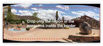
OpenCV comes with a function cv2.imshow() that displays an image in a window. The window automatically fits to the image size. You can also resize the window with the cv2.resizeWindow() function.

If you are using OpenCV 3, you have to use the function cv2.namedWindow(). This function creates a window of the specified name with the specified size.

cv2.waitKey() is a keyboard binding function. Its argument is the time in milliseconds. The function waits for specified milliseconds for any keyboard event. If you press any key in that time, the program continues. If 0 is passed, it waits indefinitely for a key stroke [1].

To read an image in Python using OpenCV, use the cv2.imread() function. imread() returns a numpy array containing the pixel values of the image [2]. You can optionally convert this array into a PIL image using img_to_pil().

The following code snippet uses these functions to display an image from file “image.png”:

import cv2

img = cv2.imread(“image.png”)

cv2.imshow(“Image”, img)

cv2.waitKey(0)

Segmenting an image is the process of partitioning it into groups of connected pixels.

Image segmentation is a very important image processing technique. It helps in extracting the meaningful information from an image and also separates different objects in an image. There are various methods for image segmentation, but the most popular one is thresholding.

Thresholding is a simple method of image segmentation where all the pixels having values above a certain threshold are assigned one value and all the pixels having values below the threshold are assigned another value. This threshold value can be fixed or it can be calculated automatically using some algorithms.

There are many advantages of using thresholding for image segmentation. One of the main advantages is that it is very easy to implement and does not require any sophisticated techniques. Another advantage is that it is relatively fast as compared to other methods such as clustering.

However, there are some disadvantages of using thresholding as well. One of the main disadvantages is that it does not always produce good results and sometimes may even lead to over-segmentation or under-segmentation of images.

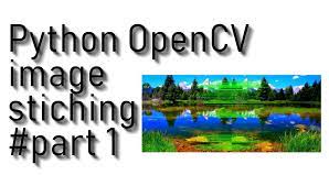
In image stitching, we create a panorama by joining together multiple images.

Image stitching is the process of combining multiple images to create a single panoramic image. By seamlessly joining together multiple photos, we can create an image with a much wider field of view than what would be possible with a single photo.

There are many different algorithms that can be used for image stitching, but the basic principle is always the same: we take multiple images and align them so that they overlap. We then blend the overlapping regions together to create a smooth, seamless transition between images.

One of the challenges in image stitching is dealing with parallax error. This occurs when two photos are taken from slightly different positions, and as a result, some objects appear shifted in one image compared to the other. To correct for this, we need to first estimate the camera’s position for each photo and then perform some geometric transformations to align the images.

Image stitching can be used to create all sorts of interesting effects, such as panoramas, high-resolution images (by combining multiple lower-resolutionimages), or even “mini-movies” by joining together successive frames from a video sequence.

To do this, we need to segment each image into overlapping regions.

We’ll use a simple function to do this, which takes an image and a window size as inputs:

def segment_image(img, window_size):

segments = []

(h, w) = img.shape[:2]

for y in range(0, h – window_size + 1):

for x in range(0, w – window_size + 1):

window = img[y:y+window_size, x:x+window_size]

segments.append(window)

return segments

We can use OpenCV to segment images automatically.

OpenCV is a computer vision library that allows us to perform image processing and computer vision algorithms. We can use OpenCV to segment images automatically. Segmentation is the process of partitioning an image into different regions. Each region can be processed separately. This is useful for many applications, such as object detection and recognition, motion estimation, and background subtraction.

show image cv2

In order to show image cv2, we need to first import the cv2 library like so:

import cv2

Once we have imported the library, we can then read in our image using the imread function. We can also specify the path to where our image is located:

image = cv2.imread(“path_to_image”)

Once we have read in the image, we can then use the imshow function to display it. We just need to pass in the name of our window and our image:

cv2.imshow(“Image”, image)

Lastly, we need to add a waitKey function in order for our image to be displayed. This is needed so that our program doesn’t immediately close after displaying the image:

cv2.waitKey(0)

matlab segment image

1. In order to segment an image using Matlab, the first step is to load the image into the software. This can be done by either using the imread command or by opening the image file in the MATLAB interface.

2. Once the image is loaded, it is necessary to convert it to a grayscale image. This can be done by using the rgb2gray command.

3. The next step is to apply a threshold to the grayscale image. This can be done by using the im2bw command. The threshold value can be specified as an input to this command.

4. After applying the threshold, the resulting binary image can be segmented into individual objects using the bwlabel command. This command will return a label matrix which can be used to identify each object in the image.

5. To obtain measurements for each object in the segmented image, the regionprops command can be used. This command will return information such as centroid, area, and bounding box for each object in the label matrix.

6. The final step is to plot the segmented image with its corresponding measurements. This can be done by using the imshow and text commands in MATLAB.

The first step is to load the images into OpenCV.

This can be done with the cv2.imread() function.

The images should be in the same directory as your Python script.

Once the images are loaded, we need to convert them to grayscale.

This can be done with the cv2.cvtColor() function.

We also need to resize the images to have uniform size.

This can be done with the cv2.resize() function.

Next, we convert the images to grayscale.

This is done by first converting the images to black and white, then averaging the channels to get a single grayscale channel.

The advantage of this approach is that it is relatively simple and does not require any sophisticated image processing algorithms.

The resulting images are still fairly high quality and can be used for many purposes such as OCR or further image analysis.

Then, we apply a threshold to the images.

This is done by first converting the image to grayscale and then using a thresholding function on the image.

The thresholding function converts the image into a binary image, where all pixels below the threshold are set to 0 (black) and all pixels above the threshold are set to 1 (white).

We can experiment with different values for the threshold to see what works best for our particular images.

After that, we find the contours in the images.

We are using the Canny edge detection algorithm for this task.

The output of the canny function is an array of boolean values (i.e., 0 or 1) that indicate whether there is an edge at that particular pixel position.

We then use the contours to find the center point of each object in the image and draw a circle around it using the cv2.circle function.

Finally, we draw the contours on the images and save them.

We start by loading the image and converting it to grayscale. We then apply a Gaussian blur to the image to smooth it out. Next, we compute the Canny edge detector on the image to find all of the edges in the image. We then find all of the contours in the image and draw them onto the original image. Finally, we save the resulting image.